A Complete Tour Of The HOME TAB in Excel Lesson-5 || Ashok TV Excel Easy & Free Tutorial

HOME TAB in Microsoft Excel Introduction Detailed Tutorial | Basic Excel Tips | Ashok Tv Excel free Tutorial

The Home Tab in Microsoft Excel is the first tab. When you open a new Excel Workbook the Home Tab is shows by default. You can do things like copy, paste, formation, alignment, inserting and deleting rows or columns, sorting and filtering numbers, applying styles and conditional formatting, finding and replacing data, auto sum, average of values and much more using the Home Tab.

Home Tab contains the 7 groups listed are as follows (from left to right on the Ribbon)

Clipboard Group

Font Group

Alignment Group

Number Group

Styles Group

Cells Group

Editing Group

In this tutorial i will explain all groups of Home Tab detailed explanation with examples also.

Clipboard

The first group is the Clipboard in Home Tab. This group contains frequently used commands: Cut, Copy, Paste and Format painter. Clipboard option allows us to collect text and graphic items and paste it.

Using these commands, you can move text from one area of your Excel sheet to another.

When you use the Cut Command, it removes the source text.

However, when you use Copy Command, it leaves the source text in place.

Using the Paste Command, you can then insert the clipboard text into the new location.

Using these commands, you can copy also formulas and formatted data from one area of the Excel worksheet to another. See given screen-shots for easy understanding how to copy, cut and paste values and formulas.

a) Using Copy and Paste Commands for Text

(1) Click A14 cell > (2) Click Copy Command > (3) Click A1 Cell > (4) Click Paste Command  

Finally, A14 cell text copy to Paste A1 cell  (Note : In A14 cell text is there.)

b) Copy as Picture

Sometimes if you can some data Copy as Picture and paste in other place, it will show data as a picture/Image.

c) Using Cut and Paste Commands for Text

 (1) Click A14 cell > (2) Click Cut Command > (3) Click A1 Cell > (4) Click Paste Command  

Finally, A14 cell text copy to Paste A1 cell. (Note : In A14 cell text is not there.)

d) Using Copy and Paste Commands for Formulas: cell

For Example: See below worksheet, I calculate the summary total of Black Shoes sales in B8 cell. Now using formula Copy command, calculate the Brown Shoes total sales. Follow given steps.

(1) Click B8 cell > (2) Click Copy Command > (3) Click C8 Cell > (4) Click Paste Command  

Explanation : Click on the cell B8 and you will, notice that in the formula bar (in left side blue rectangle) we have the formula =SUM(B3:B7) After you have selected the cell, click on copy command in the clipboard group, click on the cell C8 then click on Paste command. So it will calculate automatically Brown shoes sales total ( see updated formula in right side blue rectangle). 

e) Paste Special

If you want to paste only a specific aspect of the copied data like its formatting or value, you would use one of the Paste Special options. After you’ve copied the data, press Ctrl+Alt+V, or Alt+E+S or (Home > Paste > Paste Special) to open the Paste Special dialog box.

Explanation of Paste Special Dialog Box

Pick this option	To	Keyboard shortcut
All	Paste all cell contents and formatting.	Press A
Formulas	Paste only the formulas as entered in the formula bar.	Press F
Values	Paste only the values (not the formulas).	Press V
Formats	Paste only the copied formatting.	Press T
Comments	Paste only comments attached to the cell.	Press C
Validation	Paste only the data validation settings from copied cells.	Press N
All using Source theme	Paste all cell contents and formatting from copied cells.	Press H
All except borders	Paste all cell contents without borders.	Press X
Column widths	Paste only column widths from copied cells.	Press W
Formulas and number formats	Paste only formulas and number formats from copied cells.	Press R
Values and number formats	Paste only the values (not formulas) and number formats from copied cells.	Press U

Note: If possible, I will post details tutorial about Paste Special Command with screen-shots soon.

f) Format Painter

Like the look of a particular selection, you can apply Format Painter that look to other content in the Worksheet.

For Example: See below screenshot for easy understanding

If you want, A3 cell format like A4 cell format also. Follow these steps.

Tip: Format Painter works for Font style, Font size, colour formatting, Bold, Italic etc.

 (1) Click A3 cell > (2) Click Format Painter > (3) Click A4 cell

g) To apply the formatting in multiple places, double-click Format painter

(1) Click A3 cell > (2) Double-Click Format Painter > (3) Click A4 cell> (4) Click B7 cell> (5) Click C5 cell> (6) Click D7 cell

So finally, A3 cell format copied to A4, B7, C5 and D7 cells.

Clipboard commands Keyboard Shortcuts:

Tip-1 : Keyboard Shortcut for COPY : Ctrl + C

Tip-2 : Keyboard Shortcut for CUT : Ctrl + X

Tip-3 : Keyboard Shortcut for PASTE : Ctrl + V

Tip-4 : Keyboard Shortcut for COPY AS PICTURE : Alt+H+CP

Tip-5 : Keyboard Shortcut for PASTE SPECIAL : Ctrl+Alt+V, or Alt+E+S

Tip-6 : Keyboard Shortcut for FORMAT PAINTER : Alt+H+FP

Font Group

We use this option to change the font style and font-size. The Font group on the HOME tab provides you with access to the most commonly used commands for adjusting the fonts in your worksheets. We can make it bold, italic and underline. Also, this group contains border styles, fill color, font color.

Font – Used to select font types or change fonts from drop down list in excel.

1.Select the cell or cells or range of cells in which you wish to change the font.

2.On the HOME tab, in the Font group, click the arrow to the right of the Font command.

3.Select a font from the drop down menu what you want.

Font Size – Use this option to change the size of the font of text or numbers in cell or cells or range of cells in Excel.

1.Select the cell or cells in which you wish to change the font size.

2.On the HOME tab, in the Font group, click the arrow to the right of the Font Size command and select you wish to change the font size from drop down menu.

Increase Font Size – Used to increase font types in excel.

Decrease Font Size – Used to decrease font types in excel.

Bold – Use this option to make the text or number in cells bold in excel.

1.Select the cell or cells or cell ranges in which you wish to bold the text or number.

2.On the HOME tab, in the Font group, click the Bold command.

Italic – Use this option to make the text italic in Excel.

1.Select the cell or cells or range of cells in which you wish to italicize the text or number.

On the HOME tab, in the Font group, click the Italic command.

Underline – Use this option to underline the text or number in excel.

1.Select the cell or cells in which you wish to underline the text.

2.On the HOME tab, in the Font group, click the Underline command.

3. On the HOME tab, in the Font group, click the Underline down arrow button and select Double Underline command.

Borders – Use this option, to apply various borders type from drop down list in Excel.

1.Select the cell or cells or range of cells to which you wish to add borders.

On the HOME tab, in the Font group, click the arrow to the right of the Borders command.

Select the type of border you wish to add from the drop down menu (I select All Boarders)

Fill Color – Use this option, to change the Fill color or background color for cells in Excel.

1.Select the cell or cells or rage of cells in which you wish to change the Fill color.

2.On the HOME tab, in the Font group, click the arrow to the right of the Fill Color command.

3.Select a color from the drop down menu.

Font Color – Use this option, to apply and change font colours of selected texts or number in cell in Excel.

1.Select the cell or cells or range of cells or some of the text in cell in which you wish to change the font color of the text.

2.On the HOME tab, in the Font group, click the arrow to the right of the Font Colour command.

3.Select a colour from the drop down menu.

Alignment Group

In the Home Tab, Alignment group is third group, after the Clipboard group and the Font Group. It has the 11 buttons including in the drop down buttons.

We use this buttons to change the alignment of cell or cells’ text with Top Align, Middle Align, Bottom Align, Align Left, Center, Align Right , Orientation, Decrease Indent, Increase Indent,Wrap Text and Merge and Center.

Text within cells in Excel Worksheet can be aligned both vertically (Top, Center and Bottom) and horizontally (Left, Center and Right).

To align text vertically within a cell or cells in Microsoft Excel:

Select the cell or cells in which you wish to align the text.

On the HOME tab, in the Alignment group, click the Top Align, Middle Align or Bottom Align command:

Top Align – Use this button, to Align text of a cell or cells or range of cells at the Top.

1.Select Cells > 2.On the HOME tab, in the Alignment group, click the Top Align command
3.Result : Selected data changes to Top align like below image.

Middle Align – Use this button, to Align text of a cell or cells or range of cells at the Middle.

1.Select Cells > 2.On the HOME tab, in the Alignment group, click the Middle Align command
3.Result : Selected data changes to Middle align like below image.

Bottom Align – Use this button, to Align text of a cell or cells or range of cells at the Bottom.

1.Select Cells > 2.On the HOME tab, in the Alignment group, click the Bottom Align command
3.Result : Selected data changes to Bottom align like below image.

Align Left – Use this button, to Align text of a cell or cells or range of cells at the Left side/ Leftwards in Excel Worksheet.

1.Select Cells > 2.On the HOME tab, in the Alignment group, click the Align Left command
3.Result : Selected data changes to Left align like below image.

Center – Use this button, to Align text of a cell or cells or range of cells at the Center position in Excel Worksheet.

1.Select Cells > 2.On the HOME tab, in the Alignment group, click the Center command
3.Result : Selected data changes to Center like below image.

Align Right – Use this button, to Align text of a cell or cells or range of cells at the Right side/ Rightwards in Excel Worksheet.

1.Select Cells > 2.On the HOME tab, in the Alignment group, click the Align Right command
3.Result : Selected data changes to Right Align like below image.

Orientation – Use this button, rotates your text Horizontally or Vertically of a cell or cells or range of cells

1.On the HOME tab, in the Alignment group, click the arrow to the right of the Orientation command

2.Select orientation, what you want of your text like Angle counter clockwise, Angle Clockwise, Vertical Text, Rotate Text Up, Rotate Text Down.

3. Format cell Alignment button: On the HOME tab, in he Alignment group, click the arrow to the right of the Orientation command and select Format cell Alignment button from Drop down List.In this button you can all alignments in one window.

Decrease Indent – Use this command, to shift text of a cell closer to the cell or cells’ border in Excel worksheet.

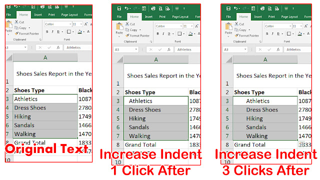
Increase Indent – Use this command, to shift text of a cell away from the cell or cells’ border in Excel worksheet. You can click Increase Indent as many times as you want to achieve the indentation you desire.

For Example, Indenting text is a way of showing that one item is a sub-item of another, as shown here.

Wrap Text

If you want long texts on multiple line in a single cell, you use Wrap Text option. Wrap text automatically or enter a manual line break. To wrap text within a cell or cells or range of cells in Excel worksheet.

Wrap text automatically : 

1.Select the cell or cells or range of cells in which you wish to wrap the text