How to use conditional formatting in Excel 2010, 2013 and 2016
Today I will explains the basics of Excel conditional formatting feature. You will learn how to create different formatting rules, how to do conditional formatting based on another cell, how to edit and copy your formatting rules in Excel 2007, 2010 2013, and 2016.
Excel conditional formatting is a really powerful feature when it comes to applying different formats to data that meets certain conditions. It can help you highlight the most important information and data in your spreadsheets and identify variances of cells' values with a quick glance.
At the same time, Conditional Formatting is often deemed as one of the most intricate and obscure Excel functions, especially by beginners. If you feel intimidated by this feature too, please don't! In fact, conditional formatting in Excel is very straight forward and easy to use, and you will make sure of this in just 5 minutes when you have finished reading this short article/tutorial.
· Excel conditional formatting basics
· Where is conditional formatting in Excel?
· How to create conditional formatting rules
· Apply several rules to one cell
· Edit conditional formatting rules
· Copy conditional formatting in Excel
· Delete formatting rules
The same as usual cell formats, you use conditional formatting in Excel to format your data in different ways by changing cells' fill color, font color and border styles. The difference is that conditional formatting is more flexible, it allows you to format only the data that meets certain criteria, or conditions.
You can apply conditional formatting to one or several cells, rows, columns or the entire table based on the cell contents or based on another cell's value. You do this by creating rules (conditions) where you define when and how the selected cells should be formatted.
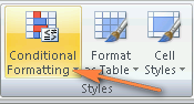
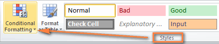
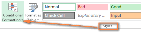
For a start, let's see where you can find the conditional formatting feature in different Excel versions. And the good news is that in all modern versions of Excel, conditional formatting resides in the same location, on the Home tab > Styles group.
Conditional formatting in Excel 2007
Conditional formatting in Excel 2010
Conditional formatting in Excel 2013 and Excel 2016
Now that you know where the conditional formatting feature is located in Excel, let's move on and see what format options you have and how you can create your own rules.
To truly leverage the capabilities of conditional format in Excel, you have to learn how to create various rule types. This will help you make sense of whatever project you are currently working on.
Conditional formatting rules in Excel define 2 key things:
· What cells the conditional formatting should be applied to, and
· Which conditions should be met.
I will show you how to apply conditional formatting in Excel 2010 because this seems to be the most popular version these days. However, the options are essentially the same in Excel 2007, 2013 and 2016, so you won't have any problems with following no matter which version is installed on your computer.
1. In your Excel spreadsheet, select the cells you want to format.
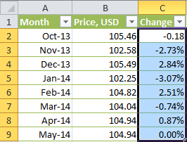
For this example, I've created a small table listing the monthly crude oil prices. What we want is to highlight every drop in price, i.e. all cells with negative numbers in the Change column, so we select the cells C2:C9.
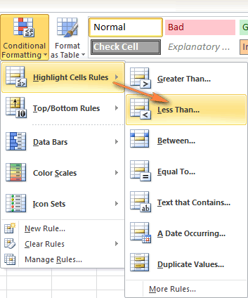
1. Go to the Home tab > Styles group and click Conditional Formatting. You will see a number of different formatting rules, including data bars, color scales and icon sets.
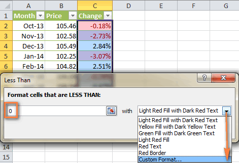
2. Since we need to apply conditional formatting only to the numbers less than 0, we choose Highlight Cells Rules > Less Than...
Of course, you can go ahead with any other rule type that is more appropriate for your data, such as:
o Format values greater than, less than or equal to
o Highlight text containing specified words or characters
o Highlight duplicates
o Format specific dates
3. Enter the value in box in the right-hand part of the window under "Format cells that are LESS THAN", in our case we type 0. As soon as you have entered the value, Microsoft Excel will highlight the cells in the selected range that meet your condition.
4. Select the format you want from the drop-down list. You can choose one of the pre-defined formats or click Custom Format... to set up your own formatting.
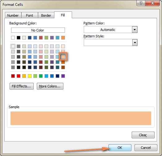
5. In the Format Cells window, switch between the Font, Border and Fill tabs to choose the font style, border style and background color, respectively. On the Font and Fill tabs, you will immediately see a preview of your custom format.
6. When done, click the OK button at the bottom of the window.
Tips:
· If you want more background or font colors than the standard palette provides, click the More Colors... button on the Fill or Font tab.
· If you want to apply a gradient background color, click the Fill Effects button on the Fill tab and choose the desired options.
· Click OK to close the "Less Than" window and check whether the conditional formatting is correctly applied to your data.
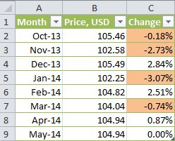
Example : As you can see in the screenshot below, our newly created conditional formatting rule works right - it shades all the cells with a negative price change.
If none of the ready-to-use formatting rules meets your needs, you can create a new one from scratch.
1. Select the cells to which you want to apply the conditional format and click Conditional Formatting > New Rule.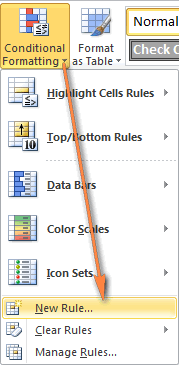
2. The New Formatting Rule dialog opens and you select the needed rule type.
Example : let's choose "Format only cells that contain" and opt to format the cell values between 60 and 70.
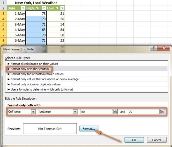
3. Click the Format... button and set up your formatting exactly as we did in the previous example.
4. Click OK twice to close the open windows and your conditional formatting is done!
Excel conditional formatting based on cell's value
In both of the previous examples, we created the formatting rules by entering the numbers. However, in some cases it makes more sense to base your condition format on a certain cell's value. The advantage if this approach is that no matter how that cell's value changes in the future, your conditional formatting will adjust automatically and reflect the data change.
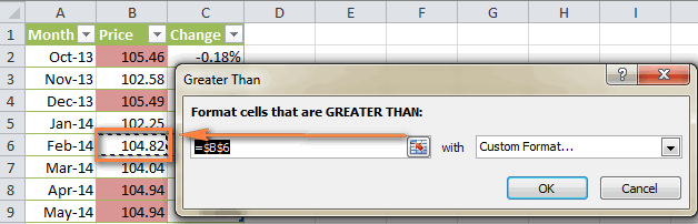
For instance, let's use the "Oil price" example again, but this time highlight all the prices in column B that are greater than February's price.
You create the rule in a similar fashion by selecting Conditional formatting > Highlight Cells Rules > Greater Than... But instead of typing a number in step 4, you select cell B6 by clicking the range selection icon as you usually do in Excel. As the result, the prices get formatted as you see in the screenshot below.
This is the simplest example of Excel conditional formatting based on another cell. Other, more complex scenarios, may require the use of formulas. And you can find several examples of such formulas along with the step-by-step instructions in this article: How to change a cell color based another cell's value.
This is how you do conditional formatting in Excel. Hopefully, these very simple rules we have just created was helpful to understand the general approach.
When using conditional formatting in Excel, you are not limited to only one rule per cell. You can apply as many rules as your project's logic requires.
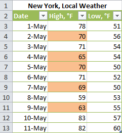
Example : let's create 3 rules for the weather table that will shade temperatures higher than 60 °F in yellow, higher than 70 °F in orange, and higher than 80 °F in red.
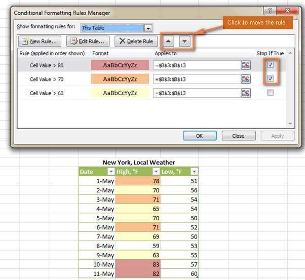
You already know how to create Excel conditional format rules of this kind - by clicking Conditional Formatting > Highlight Cells rules > Greater than. However, for the rules to work correctly, you also need to set their priority in this way:
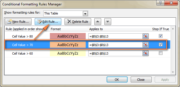
1. Click Conditional Formatting > Manage Rules... to bring up the Rules Manager.
2. Click the rule that needs to be applied first to select it, and move it to the top using the upward arrow. Do the same for the second-in-priority rule.
3. Select the Stop If True check box next to the first 2 rules because you do not want the other rules to be applied when the first condition is met.
Using "Stop If True" in conditional formatting rules
We have already used the Stop If True option in the example above to stop processing other rules when the first condition is met. That usage is very obvious and straightforward. Now let's consider two more examples where the use of the Stop If True function is not so obvious but also very helpful.
Example 1. Show only some items of the icon set
Suppose, you have added the following icon set to your sales report.
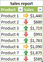
It looks nice, but a bit inundated with graphics. So, our goal is to keep only the red down arrows to draw attention to the products performing below the average and get rid of all other icons. Let's see how you can do this:
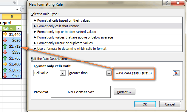
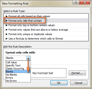
1. Create a new conditional formatting rule by clicking Conditional formatting > New Rule > Format only Cells that contain.
2. Now you need to configure the rule in such a way that it gets applied only to the values greater than the average. You do this by using the =AVERAGE() formula, as shown in the screenshot below.
Tip. You can always select a range of cells in Excel using the standard range selection icon  or type the range inside the brackets manually. If you opt for the latter, remember to use absolute cell references with the $ sign.
3. Click OK without setting any format.
4. Click Conditional Formatting > Manage Rules... and put a tick into the Stop if True check box next to the rule you have just created. And... see the result in the screenshot below : )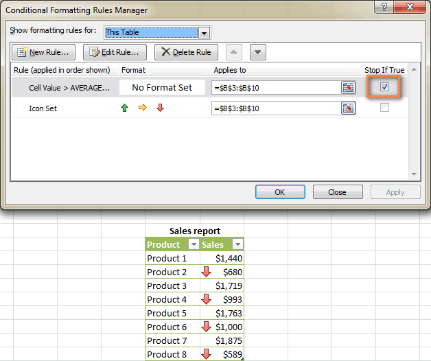
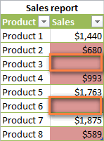
Example 2 : Remove conditional formatting from empty cells
Suppose you created the "Between" rule to highlight cells' values between $0 and $1000, as you can see in the screenshot below. But the problem is that empty cells are also highlighted.
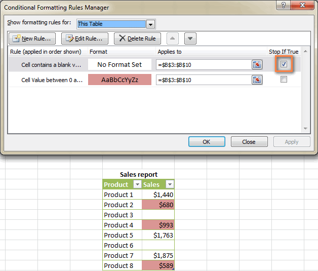
To fix this, you create one more rule of the "Format only cells that contain" type. In the New Formatting rule dialog, select Blanks from the drop-down list.
And again, you simply click OK without setting any format.
Finally, open the Conditional Formatting Rule Manager and select the Stop if true check box next to the "Blanks" rule.
The result is exactly as you would expect : )
If you've had a close look at the screenshot above, you probably noticed the Edit Rule... button there. So, if you want to change an existing formatting rule, proceed in this way:
1. Select any cell to which the rule applies and click Conditional Formatting > Manage Rules...
2. In the Conditional Manager Rules Manager dialog, click the rule you want to edit, and then click the Edit Rule... button.
3. Make the required changes in the Edit Formatting Rule window and click OK to save the edits.
The Edit Formatting Rule window looks very similar to the New Formatting Rule dialog you used when creating the rule, so you won't have any difficulties with it.
Tip. If you don't see the rule you want to edit, select This Worksheet from the "Show formatting rules for" drop-down list to display the list of all rules in your worksheet.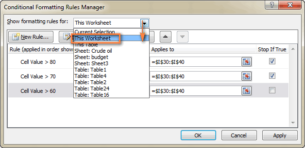
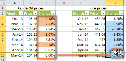
If you want to apply the conditional format you have created earlier to other data on your worksheet, you won't need to create the rule from scratch. Simply use Format Painter to copy the existing conditional formatting to the new data set.
1. Click any cell with the conditional formatting you want to copy.
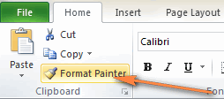
2. Click Home > Format Painter. This will change the mouse pointer to a paintbrush.
Tip. You can double-click Format Painter if you want to paste the conditional formatting in several different ranges of cells.
3. To paste the conditional formatting, click on the first cell and drag the paintbrush down to the last cell in the range you want to format.
4. When done, press Esc to stop using the paintbrush.
Note. If you've created the conditional formatting rule using a formula, you may need to adjust cell references in the formula after copying the conditional format.
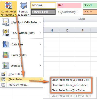
I've saved the easiest part for last : ) To delete a rule, you can either:
· Open the Conditional Manager Rules Manager (as you remember, you open it via Conditional Formatting > Manage Rules...), select the rule and click the Delete Rule button.
· Select the range of cells, click Conditional Formatting > Clear Rules and choose one of the available options.
Now you have basic knowledge of Excel conditional format. In the next article, we will focus on more advanced features that will help you push conditional formatting in your spreadsheets far beyond its traditional uses
Comments
Post a Comment